INDEX MATCH: A Practical Guide to Flexible Excel Lookups

Key takeaways

• INDEX MATCH combines two Excel functions to perform flexible lookups by using MATCH to find the position of a value and INDEX to return the corresponding result. It is a popular alternative to VLOOKUP for more advanced lookup tasks.

• You can use INDEX MATCH to perform left lookups, two-way lookups, and other advanced lookup tasks in Excel worksheets.

• INDEX MATCH works in two ways: MATCH first identifies the position of a lookup value, and INDEX uses that position to return the related data from another range.

INDEX and MATCH differ from VLOOKUP in that they use numeric positions to retrieve data. See how INDEX MATCH can be applied to common Excel lookup tasks with practical examples and troubleshooting guidance.

Afterward, if you’re ready to level up your data analysis skills, consider enrolling in the Excel Skills for Data Analytics and Visualization Specialization. You’ll have the opportunity to learn how to analyze complex data sets using Excel, create interactive dashboards, automate data transformation, and more.

What is INDEX MATCH in Excel?

The INDEX and MATCH functions in Excel are popular ways of handling advanced lookups. Because the INDEX function can return values from virtually anywhere in a range, it is widely used in more complex formulas. When combined, the INDEX MATCH function can replace HLOOKUP and VLOOKUP when you need a more flexible way to find and return data [1].

Why use INDEX MATCH instead of VLOOKUP?

INDEX MATCH is more flexible than VLOOKUP because it can retrieve values from any direction and works with both vertical and horizontal ranges. The advantages are:

1) Supports left lookups—retrieves values to the left of the lookup column

(2) Works with both vertical and horizontal ranges

(3) Uses numeric positions (MATCH finds position, INDEX returns value), offering more flexibility than VLOOKUP's fixed column-index approach.

While it requires two functions, it offers a flexible and customizable solution for a wide range of lookup tasks. Unlike VLOOKUP, INDEX and MATCH use numeric positions to locate data. MATCH identifies the position of a value, and INDEX returns the value at that position. Although this approach requires a little more setup, it provides greater flexibility when working with vertical or horizontal ranges.

How does an INDEX MATCH work?

INDEX MATCH works by combining the INDEX and MATCH functions to look up and return data in an Excel worksheet. The INDEX function returns the value stored at a specified position within a range. The syntax is =INDEX(array, row_num, [column_num]).

In contrast, the MATCH function searches a range for a specified value and returns its position rather than the value itself. The syntax is =MATCH(lookup_value, lookup_array, [match_type]). The match_type argument defines how Excel compares lookup_value with the values in lookup_array.

INDEX MATCH formula

You can use INDEX and MATCH separately or use them together for more advanced searches. A combination of INDEX and MATCH formulas looks like this:

=INDEX(return_array, MATCH(lookup_value, lookup_array, [match_type]))

The match_type can take the value -1, 0, or 1. If you enter -1, MATCH finds the smallest value that is greater than or equal to your lookup_value. To find the first value that is exactly equal to your lookup_value, enter 0.

Practical use cases

With INDEX and MATCH, you can perform vertical and horizontal lookups, two-way lookups, left lookups, and case-sensitive lookups. It is especially useful when you need to retrieve multiple attributes from a table or data set using a single lookup value.

A simple example is using INDEX MATCH to retrieve information from a movie database. By entering a movie title, the formula can return details such as its release year, ranking, or other information. The process begins with the MATCH function, which finds the row containing the movie title you are looking for, then the INDEX function uses that row number to return the corresponding value.

For another example, imagine you have a spreadsheet containing office location numbers and need to identify which employees work in each location. Rather than manually searching through a large data set, you can use a lookup formula such as INDEX MATCH to quickly return the corresponding employee information.

INDEX MATCH example

To better understand how INDEX MATCH works, try creating a simple practice worksheet that looks up a person's name and age and returns a related value from the table. Working through a small data set can help you see how the INDEX and MATCH functions work together to retrieve information.

First, create your table.

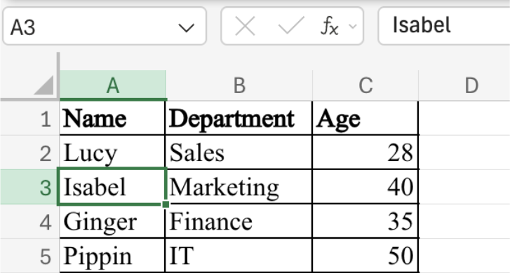
If you want to find Isabel's age, you can use the following formula:

=INDEX(C2: C5, MATCH("Isabel", A2: A5, 0))

This formula searches for Isabel in the “Name” column and returns the matching value from the “Age” column. Below is a breakdown of the formula:

“Isabel” is in A3, which is within the lookup range A2: A5

MATCH("Isabel", A2: A5, 0) returns 2 as Isabel is the second item in the range. Note that the match type “0” specifies that the lookup value must match exactly.

Finally, INDEX(C2: C5, 2) returns the second value in the C2: C5 range, which is 40.

If you replace "Isabel" with "Lucy", the same formula returns Lucy's age instead.

Read more: How to Create a Dummy Variable in Excel: A Step-by-Step Guide

INDEX MATCH vs. newer Excel options: Is INDEX MATCH still useful?

As Excel has evolved, Microsoft has introduced newer lookup functions, such as XLOOKUP and XMATCH. Even with these newer options, INDEX MATCH remains a valuable skill because it works in all versions of Excel and is still used in many existing workbooks. Learning INDEX MATCH can help you work with a wider range of Excel files and understand formulas you may encounter in the workplace.

Troubleshooting tips

If your INDEX MATCH formula does not return the expected result, the issue could be a small mistake in the formula or the data. Checking the following common problems can help you identify and fix the error. Frequent issues include:

• Exact match vs. approximate match: The MATCH function supports both exact and approximate matches. Using the wrong match type can cause the formula to return unexpected results, especially when using an approximate match with unsorted data.

• Mismatched ranges: The array used by INDEX and the lookup array used by MATCH should refer to the same records. If the ranges are different sizes or are not aligned, the formula may return an error or the wrong value.

• Not using the array formula: With older versions of Microsoft 365, using INDEX and MATCH together requires using an array formula. Without it, you may get a #VALUE! error, which you can fix by pressing CTRL+SHIFT+ENTER to wrap your formula in the required brackets. However, if you have the current version of Microsoft 365, you only need to press ENTER [2].

• Missing values: If MATCH cannot find the lookup value, it returns a #N/A error. Hidden spaces, unexpected characters, or inconsistent data types can prevent Excel from finding a value that appears to be present.

• Incorrect references: Incorrect cell references can also cause INDEX MATCH to fail. Double-check that each reference points to the intended cells, especially after copying or editing the formula or adding or deleting columns.

Explore our free resources for Excel

Subscribe to Career Chat, our weekly LinkedIn newsletter for career advice. Continue learning more about Excel with some of our free resources:

• Bookmark for future reference: Excel Formulas Cheat Sheet

• Watch on YouTube: Excel Range Names + Find & Replace (Fast Navigation)

• Take a quiz: Microsoft Excel Skill Assessment

With Coursera Plus, you can learn and earn credentials at your own pace from over 350 leading companies and universities. With a monthly or annual subscription, you’ll gain access to over 10,000 programs. Just check the course page to confirm your selection is included.